


Introduction
Effective Calibration Curve Design and Regression Weighting in LC-MS/MS bioanalysis requires matching the mathematical order of the calibration function and its inverse-variance weighting scheme—typically linear or quadratic regression paired with 1/x2 weighting—to the empirical heteroscedasticity and upper-end saturation behavior of the mass spectrometric detector. Because quantitative bioanalytical assays routinely span three to four orders of magnitude in complex matrices such as plasma, serum, urine, and cerebrospinal fluid, mis-specifying either the model order or the weight propagates systematic bias into lower limit of quantification (LLOQ) and quality control (QC) accuracy, distorting the concentration–time data used to derive peak concentration (Cmax) and area under the curve (AUC) metrics.
High-sensitivity triple-quadrupole platforms can reach detection limits in the picogram-per-milliliter range, yet greater ionization and detection efficiency narrow the proportional dynamic window at the upper limit of quantification (ULOQ). Regulated bioanalytical laboratories—such as contract research organizations including ResolveMass Laboratories Inc. executing GLP and GMP studies across FDA, EMA, and Health Canada jurisdictions—must characterize calibration variance empirically during method development and lock the regression equation and weighting rule a priori before analyzing clinical or toxicokinetic study samples.
Explore integrated chemistry and bioanalytical CRO capabilities to support analytical programs with coordinated scientific expertise.
Share via:
Quick Summary:
- Match the model to the detector. LC-MS/MS assays span 3–4 orders of magnitude, so the regression order (linear or quadratic) and the weighting must reflect how the detector actually behaves. Getting either wrong biases LLOQ and QC accuracy, and that bias carries into Cmax and AUC.
- Unweighted OLS fails across wide ranges. Signal error grows with concentration (heteroscedasticity), so high standards dominate the slope and distort the low end. Confirm it with residual plots, which show a funnel shape, and with an F-test or ANOVA comparing LLOQ and ULOQ variance.
- 1/x² is the standard weighting. It corrects for proportional error, where %CV stays constant, and gives the best LLOQ accuracy. It is preferred over 1/y² because x (nominal concentration) is treated as known without error. Zero samples cannot be included in 1/x or 1/x² fits.
- Choose the model by Σ|%RE|, not R². A high R² can hide large low-end bias. Compare candidate models using back-calculated %RE, the spread of weighted variances, and standardized residual plots. Use a partial F-test or Mandel’s test to decide on a quadratic.
- Don’t force through zero, and don’t switch after the fact. A free intercept reveals interference, carryover, or IS contamination. Changing the weighting or model order to rescue a failed run is never acceptable.
- Fix upper-end curvature at the instrument first. Bending usually comes from detector saturation, ionization competition, or isotopic cross-talk with the SIL-IS. The fixes are lower detector gain, alternate SRM transitions, dilution or smaller injections, cleaner extraction, and checking SIL-IS purity and isotope overlap. Use weighted quadratic regression only when it is statistically justified.
- Follow ICH M10 a priori. Each run needs a blank, a zero, and at least 6 non-zero standards, with at least 75% of standards within ±15% (±20% at LLOQ). The model and weighting must be locked before study samples are analyzed. Accurate low-end quantitation protects AUC and t½, and controlling saturation protects Cmax.
Why Unweighted Ordinary Least Squares Fails Across Wide Dynamic Ranges
Unweighted ordinary least squares (OLS) regression fails across multi-order-of-magnitude LC-MS/MS calibration spans because absolute detector signal variance increases with analyte concentration (heteroscedasticity), allowing upper-end standards to exert disproportionate leverage on the slope and induce severe percentage bias at the LLOQ.
Simple unweighted linear regression (y = a + bx) presupposes homoscedasticity: for every nominal concentration x, the subpopulation of measured detector responses y is normally distributed around the regression line with an identical variance σ2 across the entire working range. In chromatographic bioanalysis spanning more than one order of magnitude—and commonly 1,000-fold or three to four orders of magnitude in clinical studies—absolute standard deviation (SD) typically increases proportionally with concentration while relative standard deviation (%CV or %RSD) remains roughly constant. Because OLS minimizes unweighted squared vertical residuals equally across all standards, a minor absolute error at a 1,000 ng/mL ULOQ outweighs an equivalent percentage deviation at a 1 ng/mL LLOQ by orders of magnitude, pivoting the fitted line away from the low-concentration anchors.
Bioanalysts must verify heteroscedasticity statistically rather than assuming equal variance or applying weights by convention. Two complementary diagnostic checks confirm unequal variance across the calibration span:
- Residual Dispersion Plots: Plotting raw residuals (R = Sexp − Sint, where Sexp is the observed detector signal and Sint is the interpolated regression signal) against nominal concentration reveals a widening funnel pattern under heteroscedastic conditions, whereas an appropriately weighted model yields random scatter centered on zero.
- Variance-Ratio F-Test: Replicate measurements (n per level) at the lowest concentration (s12) and highest concentration (s22) are evaluated using the experimental variance ratio:
Fexp = s22 / s12
Under the statistical validation framework detailed by Almeida et al. (2002), homoscedasticity is rejected whenever Fexp exceeds the tabulated critical value Ftab(f1, f2; 0.99) at a 99% confidence level for f1 = f2 = n − 1 degrees of freedom. Similarly, clinical bioanalytical recommendations published in Annals of Laboratory Medicine apply an ANOVA F-test comparing variance at the lowest and highest calibrator concentrations, classifying data as significantly heteroscedastic whenever P < 0.05 and formally requiring weighted regression.
If calibration performance is inconsistent, review common bioanalytical method validation failures to identify potential sources of analytical bias and method instability.
Statistical Frameworks for Calibration Curve Design and Regression Weighting
Rigorous Calibration Curve Design and Regression Weighting counteracts upper-concentration leverage by multiplying each squared residual by a weighting factor wi inversely proportional to its error variance, balancing relative accuracy uniformly from LLOQ to ULOQ.
Comparing Weighting Schemes in LC-MS/MS Bioanalysis
Among commonly evaluated empirical weights (1/x0.5, 1/x, 1/x2, 1/y, and 1/y2), 1/x2 is the most widely recommended choice for LC-MS/MS bioanalysis because it directly compensates for proportional error where SD scales linearly with concentration without propagating dependent-variable measurement noise into the weights.
In exact statistical theory, optimal weighted least squares assigns each calibration level a weight equal to the reciprocal of its true response variance (wi = 1/σi2), which requires extensive replicate determinations at every standard concentration. In routine bioanalytical practice, empirical inverse functions of nominal concentration (x) or instrument signal (y) serve as practical proxies. When raw signal variance grows linearly with concentration (σi2 ∝ xi), applying 1/x weighting produces uniform weighted variances across the calibration range. More frequently in LC-MS/MS assays, proportional error dominates (σi ∝ xi), meaning variance scales with the square of concentration (σi2 ∝ xi2) and 1/x2 weighting delivers constant weighted variance and minimal LLOQ relative error. In an Analytical Chemistry evaluation of six weighting options (unweighted, 1/x0.5, 1/x, 1/x2, 1/y, and 1/y2) across linear and quadratic LC-MS/MS calibration models, Gu et al. (2014) examined the impacts of incorrect weights on curve stability and data quality, supporting 1/x2 as the standard bioanalytical LC-MS/MS weighting factor.
Although both 1/x2 and 1/y2 often produce lower relative residuals and lower quantification limits than unweighted or 1/x fits, standard regression equations treat x as the fixed nominal independent variable known without error (assuming accurate gravimetric weighing and volumetric dilution), whereas y is the dependent instrument response measured with experimental error. Consequently, 1/x2 is widely preferred in regulated LC-MS/MS laboratories while 1/y and 1/y2 remain less common alternatives. Notably, zero-concentration samples (x = 0) must never enter regressions weighted by 1/x or 1/x2 because division by zero is mathematically undefined. As an alternative to explicit weighting, a ChemRxiv preprint evaluating a natural-log (LN) model that fits ln(concentration) against ln(peak area) showed that log-space residuals approximate relative error (ε = ln(1 + RE) ≈ RE) across wide linear ranges, although performance still degrades once upper standards enter detector saturation.
| Weighting or Transformation Scheme | Underlying Error Variance Assumption | Mathematical Weight (wi) | Primary Impact on LC-MS/MS Fit | Key Analytical Caveats and Limitations |
|---|---|---|---|---|
| Unweighted (OLS) | Homoscedastic (σi2 = constant) | 1 | Minimizes absolute vertical residuals; upper standards dominate slope. | Induces unacceptable low-end bias and elevated LLOQ %RE over more than one order of magnitude. |
| Square-Root Inverse Concentration | Sub-linear variance growth (σi2 ∝ xi0.5) | 1/xi0.5 | Moderately reduces high-concentration leverage. | Typically yields higher total relative error than 1/x or 1/x2 across wide spans. |
| Inverse Concentration | Variance proportional to concentration (σi2 ∝ xi) | 1/xi | Equalizes weighted variances when raw variance increases linearly with x. | Excludes x = 0 from regression; under-protects LLOQ when proportional error (%CV constant) dominates. |
| Inverse Squared Concentration | Proportional error / constant %CV (σi2 ∝ xi2) | 1/xi2 | Minimizes relative percentage error uniformly; strongest LLOQ accuracy. | Excludes x = 0 from regression; relies on high gravimetric/volumetric precision at low standards. |
| Inverse Signal / Squared Signal | Variance proportional to y or y2 | 1/yi or 1/yi2 | Lowers LLOQ bias and relative residuals similarly to 1/x2 in stable linear assays. | Weights incorporate dependent-variable measurement error in y; less commonly recommended than 1/x2. |
| Natural-Log Transformation (LN Model) | Constant relative error in log-space | Unweighted on ln(y) vs. ln(x) | Residuals directly approximate relative error (≈ RE) across linear spans. | Reported in preprint literature; loses accuracy at detector saturation without algorithmic range trimming. |
Diagnostic Metrics for Calibration Curve Design and Regression Weighting Selection
Selecting an optimal model during Calibration Curve Design and Regression Weighting requires evaluating the sum of absolute relative errors (Σ|%RE|), the dispersion of weighted normalized variances across levels, and standardized residual plots rather than relying on correlation (r) or determination (R2) coefficients.
Treating R2 > 0.99 or 0.995 as sufficient proof of calibration validity is a well-documented statistical pitfall. Because R2 measures overall explained variance dominated by upper-end magnitudes, a multi-order curve can post a high R2 while hiding substantial percentage bias near the LLOQ. An illustrative benchmark dataset (din) in the envalysis R package implementing Almeida et al.’s (2002) selection procedure demonstrates this disconnect: 1/x2 weighting achieved the lowest sum of absolute relative errors (0.6109) even though its adjusted R2 (0.9841) was slightly lower than 1/x weighting (sum relative error 0.6929; adjusted R2 0.9863), while both improved substantially over unweighted regression (sum relative error 0.7978; adjusted R2 0.9830). Likewise, an evaluation in LCGC showed the sum of relative errors dropping from 12.23 with no weighting to 3.39 at 1/x0.5 before plateauing at lower error levels under stronger inverse weights.
Bioanalysts should rely on three quantitative diagnostics in tandem:
- Back-Calculated Relative Error (Σ|%RE|): Compute percentage relative error at every calibration standard:
%RE = [(Cexp − Cnom) / Cnom] × 100
where Cexp is the back-calculated concentration and Cnom is the nominal concentration. The appropriate model yields the lowest Σ|%RE| while keeping individual standard deviations within a tight band around zero.
- Uniformity of Weighted Normalized Variances: In a systematic model-selection workflow benchmarked across 50 simulated datasets per calibration model (parameterized from 50 experimental LC-MS/MS analytes) and applied to cocaine and naltrexone assays, replicate variance at each concentration level is multiplied by each candidate weight (unweighted, 1/x, and 1/x2) and normalized. Because the true weighting factor equalizes weighted variances across all concentrations, selecting the weight that yields the smallest spread among weighted normalized variances provides an objective double-check of F-test findings.
- Standardized Residual Plots: Plotting weighted or standardized residuals against nominal concentration exposes subtle curvature or systematic bias masked by R2.
| Diagnostic Metric | Mathematical Basis | Selection Criterion | Common Failure Prevented |
|---|---|---|---|
| Variance-Ratio F-Test / ANOVA | Ratio of ULOQ to LLOQ replicate variances (s22 / s12) | Fexp > Ftab (99% CI) or ANOVA P < 0.05 | Prevents applying unweighted OLS to heteroscedastic data. |
| Sum of Absolute Relative Errors (Σ|%RE|) | Sum of |(Cexp − Cnom) / Cnom| × 100 | Lowest total Σ|%RE| across all calibrators | Eliminates R2-driven selection bias favoring ULOQ over LLOQ. |
| Spread of Weighted Normalized Variances | Variance across levels of normalized Wi · si2 | Smallest dispersion across concentration levels | Distinguishes 1/x from 1/x2 objectively without analyst subjectivity. |
| Partial F-Test / Mandel’s Test | Comparison of quadratic vs. linear regression sum of squares | Statistically significant reduction in residual sum of squares | Prevents overfitting random noise or forcing curved data onto straight lines. |
| Standardized Residual Plot | Visual plot of (Sexp − Sint) or standardized error vs. x | Random distribution centered on zero with no funnel or curvature | Reveals unmodeled non-linearity and bias hidden by R2 > 0.99. |
For a broader understanding of regulatory expectations, consult the ICH M10 bioanalytical method validation guidelines when establishing validation and calibration acceptance criteria.
Avoiding Origin Forcing and Post-Hoc Weight Switching
Forcing a calibration curve through the origin (0,0) and changing weighting factors or regression orders post-hoc to pass failing analytical batches compromise accuracy and violate regulated bioanalytical principles.
Leaving the y-intercept unforced (y = a + bx) preserves critical analytical quality control: as highlighted in chromatography literature and practitioner discussions, forcing through zero can degrade overall curve quality, whereas retaining a free intercept exposes background signals from matrix interferences, carryover, or trace unlabeled contamination in the internal standard. Proper inverse-concentration weighting (1/x or 1/x2) stabilizes the lower end of the curve naturally without discarding the intercept. Equally important, Annals of Laboratory Medicine bioanalytical guidelines emphasize that weighting factors must never be chosen merely because QC recoveries pass in an isolated validation batch—an improperly weighted model can coincidentally pass ±15% QC acceptance criteria in one run while failing unpredictably later. Switching weighting factors (for example, adding 1/x2 weighting) or converting a linear model into a quadratic equation during production sample analysis strictly to rescue a failed calibration curve must never be done.
Linear vs. Quadratic Regression: Saturation Physics and Isotopic Cross-Talk
Downward curvature at the upper end of LC-MS/MS calibration curves arises primarily from electron multiplier detector saturation in high-sensitivity instruments, electrospray ionization (ESI) charge competition, or isotopic cross-signal contribution involving the stable isotope-labeled internal standard (SIL-IS)—physical issues that should be corrected instrumentally before adopting a quadratic equation.
Detection Capacity Limited vs. Ionization Capacity Limited Mechanisms
Modern high-sensitivity triple-quadrupole platforms operate predominantly as Detection Capacity Limited (DCL) systems in which detector saturation occurs before ESI ion suppression, breaking the internal standard’s ability to restore calibration linearity.
Distinguishing between ionization and detection bottlenecks dictates the correct analytical fix. Older, lower-sensitivity LC-MS platforms typically behaved as Ionization Capacity Limited (ICL) systems: at high concentrations, ESI ion suppression occurred prior to detector ceiling limits, and a coeluting SIL-IS experienced identical suppression, preserving a linear analyte-to-IS peak area ratio. Conversely, modern high-sensitivity LC-MS/MS instruments act as DCL systems where high ion flux saturates the detector well before major ESI suppression occurs. Mechanistically, DCL saturation creates disproportionate growth between peak area (PA) and peak height (PH): peak height hits a physical ceiling while peak area continues expanding slightly, causing the PA/PH ratio and unit response to drop. Because the high-concentration analyte hits the ceiling while the constant-concentration SIL-IS remains inside its linear detection zone, the analyte/IS response ratio curves downward. Additional high-concentration non-linearity in ESI-MS can result from dimer or cluster ion formation and matrix-dependent ionization effects.
Bioanalytical consensus recommends mitigating physical causes of non-linearity during method development to preserve a linear response wherever practical. Analysts can expand the Near-Linear Response Range (NLRR) using four targeted interventions:
- Lowering Detector Gain: Reducing LC-MS detector gain pulls high-concentration responses below the peak height ceiling without altering chromatographic selectivity.
- Using Less-Optimal SRM Transitions: Monitoring secondary Selected Reaction Monitoring (SRM) transitions or adjusting collision energy and dwell times selectively dampens excessive ion current for abundant analytes.
- Reducing On-Column Mass Load: Increasing the sample extraction dilution factor or injecting smaller sample volumes restores proportional peak growth at the ULOQ.
- Removing Coeluting Matrix Suppressors: Replacing non-selective cleanups with liquid-liquid extraction (LLE), salting-out assisted LLE (SALLE), or mixed-mode solid phase extraction (SPE) eliminates coeluting glycerophosphocholines (characteristic fragment m/z 184) and lysophosphatidylcholines (m/z 104) that distort ionization in crude extracts containing high phospholipid and salt loads.
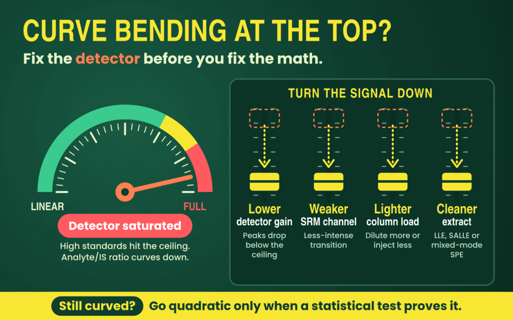
When wide clinical exposure profiles cannot fit inside the expanded NLRR, weighted quadratic regression (y = ax2 + bx + c) is scientifically valid provided model order is verified statistically through a partial F-test or Mandel’s test. Simulations based on experimentally obtained calibration curves showed a 12% average improvement in QC accuracy when applying a quadratic model to curved, uniformly weighted data rather than forcing a linear fit. Similarly, mechanistic evaluation of standard A4 demonstrated that 1/x-weighted quadratic regression extended the calibratable upper range from 800 nmol/L (linear limit) to 2,600 nmol/L. Even so, quadratic models carry firm constraints: unknown concentrations exceeding the ULOQ cannot be extrapolated reliably and require validated dilution, and pushing calibrators deep into the flat peak-height saturation ceiling still defeats quadratic accuracy.
Mitigating Isotopic Cross-Talk and SIL-IS Interference
Isotopic cross-talk degrades calibration linearity at opposite extremes: naturally occurring heavy isotopes in sulfur-, chlorine-, or bromine-containing analytes spill into the SIL-IS MRM transition to depress upper standards, whereas unlabeled impurities in the SIL-IS inflate response near the LLOQ.
When an analyte contains atoms with prominent heavy isotopes such as sulfur, chlorine, or bromine, natural analyte isotopologues overlap the mass transition of the SIL-IS, progressively inflating the internal standard peak area at high analyte concentrations and inducing downward curve non-linearity. In a peer-reviewed investigation of flucloxacillin (analyte precursor m/z 454) across Waters Xevo TQ-S and Shimadzu 8050 instruments, monitoring the primary SIL-IS transition (m/z 458 → 160) at 0.7 mg/L generated assay biases up to 36.9% due to analyte isotope spillover. Switching to a less abundant SIL-IS isotope transition (m/z 460 → 160) free of natural analyte overlap lowered bias to 13.9% at 0.7 mg/L, while increasing SIL-IS concentration to 14 mg/L reduced bias to 5.8%—a strategy successfully extended to cefotaxime, cefepime, and cefazolin.
Reverse cross-signal interference arises when an SIL-IS contains trace unlabeled analyte or suffers isotopic instability in aqueous solutions (such as poor stability in water-containing solvents proposed for 13C,D3-rofecoxib), generating false analyte peaks in zero samples. A 2025 Analytical Chemistry investigation also documented parent-drug contamination inside commercial metabolite standards (such as morphine glucuronides containing parent morphine) and interconversion between rifampicin and its derivative; to keep blank interference ≤20% of the analyte LLOQ, bioanalysts must pre-screen SIL-IS isotopic purity, lower metabolite ULOQs where cross-contribution occurs, or prepare separate calibration curves.
Evaluate matrix effects in LC-MS/MS bioanalysis to better understand how matrix-related interference can affect response consistency and quantitative accuracy.
Regulatory Architecture Under ICH M10, FDA, and EMA Frameworks
Under the harmonized ICH M10 guideline (finalized Step 4/5 in May 2022 and adopted by the US FDA in November 2022), every chromatographic analytical batch requires a blank sample (free of analyte and IS, often termed a double blank), a zero sample (blank spiked with IS), and at least six non-zero calibration standard levels—excluding blanks from regression calculations—with at least 75% of standards passing within ±15% of nominal concentration (±20% at the LLOQ).
A central pillar of ICH M10 is “a priori” standardization: the regression model, weighting function, standard rejection criteria, and chromatographic integration rules must be defined in validation protocols and SOPs before study sample analysis begins. When non-linear models such as quadratic regression are selected, additional standard concentrations beyond the six-level minimum are expected to define curvature reliably. Running duplicate calibration curves bracketing the analytical batch—or interspersing single-replicate calibrators across the run—mitigates within-batch sensitivity drift. Quality control samples (LLOQ, Low ≤3× LLOQ, Medium 30–50% of range, and High ≥75% of ULOQ) must be prepared from a separate stock solution or independent weighing during initial accuracy and precision validation so preparation errors in calibrator stocks do not go undetected.
ICH M10 harmonized longstanding operational differences between legacy EMA (2011) and FDA (2018) bioanalytical guidances—distinctions summarized below alongside legacy comparison literature.
| Regulatory Parameter | ICH M10 Chromatographic Requirement (2022–Present) | Legacy EMA (2011) vs. FDA (2018) Context |
|---|---|---|
| Calibration Curve Structure | Blank sample (no analyte/IS), zero sample (blank + IS), and ≥6 non-zero levels including LLOQ and ULOQ; blank and zero excluded from fit. | EMA strictly specified ≥6 non-zero levels with a 75% pass rule; FDA required ≥6 non-zero calibrators with less prescriptive percentage wording. |
| Standard Accuracy & Pass Threshold | ±15% of nominal (±20% at LLOQ); ≥75% of standards across ≥6 levels must pass. | Harmonized around the legacy EMA 75% (e.g., 6 of 8 standards) benchmark. |
| LLOQ Sensitivity & Interference | Validation requires ≤±20% bias and ≤20% CV across ≥5 replicates in ≥3 runs over ≥2 days; blank interference ≤20% of LLOQ and ≤5% of IS. | EMA historically required S/N ≥5:1 at LLOQ; FDA emphasized analytical response and reproducibility. |
| Anchor Calibration Standards | Defined for Ligand Binding Assays (below LLOQ or above ULOQ to assist curve fit), excluded from acceptance counts; chromatographic curves span LLOQ–ULOQ. | FDA historically permitted anchor points more flexibly to support curve modeling. |
| OOS Standard Rejection | Reject failing standard and re-regress; if LLOQ is rejected, the next lowest passing standard becomes the run’s new lower limit. | Required predefined SOP rules and audit trails covering both accepted and failed runs. |
| Regression & Weighting Reporting | For comparative BA/BE studies, 100% of run summary sheets of accepted and failed runs must report calibration curve, regression, weighting function, response ratio, and integration type. | EMA reviews historically scrutinized statistical weighting comparisons and residual plots more heavily than FDA reviews. |
| Matrix Matching & Selectivity | Calibrators in study matrix (or justified surrogate for rare/endogenous matrices); selectivity and matrix effects across ≥6 lots (plus hemolyzed/lipemic) within ±15% accuracy and ≤15% CV. | Both agencies required multi-lot matrix assessment, with EMA favoring explicit matrix factor (MF) evaluations. |
| In-Study QC & ISR Acceptance | ≥67% (2/3) of total QCs and ≥50% per level within ±15%; ISR requires ≥67% of repeats within ±20% difference. | EMA mandated 10% ISR (minimum 10 samples) for pivotal PK/TK; FDA strongly recommended ISR without a fixed sample percentage. |
Review the EMA versus FDA bioanalytical method validation differences to understand how regional expectations evolved into the harmonized ICH M10 framework.
Operational Workflow for Calibration Curve Design and Downstream PK Integrity
Executing a defensible Calibration Curve Design and Regression Weighting strategy requires a sequential development-to-validation workflow that safeguards downstream pharmacokinetic (PK) accuracy at both peak exposure (Cmax) and terminal elimination (AUC0–∞). Specifically, controlling upper-end detector saturation protects peak concentration measurements near Tmax, while minimizing low-end relative error preserves the terminal elimination rate constant (ke) and extrapolated exposure.
- Map Clinical Range and Calibrator Spacing: Define LLOQ and ULOQ around anticipated study concentrations, preparing 6–8 or more non-zero standards spaced to cover the dynamic range (adding intermediate levels if quadratic curvature is expected).
- Verify Matrix Selectivity and Carryover: Screen blank matrix from at least six individual lots—plus lipemic and hemolyzed sources—to verify interfering peaks remain ≤20% of analyte LLOQ response and ≤5% of IS response, and confirm blank carryover following the ULOQ meets identical limits.
- Eliminate Saturation and Isotopic Cross-Talk: Inspect peak-area-to-peak-height (PA/PH) ratios at upper calibrators and test SIL-IS purity and isotope overlap; tune detector gain, collision energy, injection volume, or SIL-IS transitions first to maximize linearity.
- Confirm Heteroscedasticity and Select Weighting: Measure replicate standards across the range, prove unequal variance via the LLOQ/ULOQ F-test (Fexp > Ftab) or ANOVA (P < 0.05), and compare 1/x versus 1/x2 using Σ|%RE|, spread of weighted normalized variances, and residual plots.
- Validate Model Order Statistically: Apply a partial F-test or lack-of-fit test to verify whether quadratic curvature offers statistically significant improvement over a linear equation, locking both order and weighting factor in the validation plan.
- Challenge Accuracy, Precision, and Dilution Integrity: Analyze independent-stock QCs (LLOQ, Low, Medium, High; ≥5 replicates per level across ≥3 runs over ≥2 days) and dilution integrity QCs above the ULOQ to confirm bias within ±15% (±20% at LLOQ) and precision ≤15% CV (≤20% at LLOQ).
- Monitor In-Study Slope and SIL-IS Stability: Bracket study runs with duplicate calibration curves or interspersed standards alongside duplicate QCs (≥5% of study sample count), and track SIL-IS response trends across every unknown specimen to catch unanticipated matrix shifts or slope drift.
Every upstream calibration choice directly governs the pharmacological integrity of the final study dataset. If unmitigated DCL detector saturation depresses the upper calibration response without proper modeling, high-concentration accuracy breaks down, directly compromising measured Cmax near Tmax. Conversely, along the terminal elimination phase as concentrations approach the LLOQ, unweighted OLS or insufficient low-end weighting induces disproportionate %RE; because terminal elimination rate constants (ke), elimination half-life (t1/2), and extrapolated exposure depend on accurate quantitation of the last measurable time points, LLOQ bias propagates directly into total AUC estimates.
AUC0–∞ = AUC0–t + Ct / ke
Establishing a robust, well-weighted LLOQ also enables the method to monitor >80% of the total PK profile AUC while supporting reproducible Incurred Sample Reanalysis (ISR) performance across peak and elimination phases.
Explore bioanalytical stability testing to support reliable analyte measurement throughout sample collection, storage, processing, and analysis.
Conclusion
Achieving precision in Calibration Curve Design and Regression Weighting requires treating statistical regression as a representation of the underlying mass spectrometric behavior rather than relying on automated software defaults. By demonstrating heteroscedasticity through variance-ratio F-tests and normalized variance distribution, replacing conventional reliance on R2 with Σ|%RE| calculations and residual diagnostics, correcting DCL detector saturation and SIL-IS isotopic cross-talk at the instrument level, and following predefined ICH M10 validation requirements, bioanalytical teams can maintain quantitative reliability across the entire concentration range, from terminal LLOQ measurements to peak Cmax concentrations.
Whether developing highly sensitive small-molecule PK methods, multi-metabolite assays, or complex peptide workflows using advanced triple-quadrupole instruments such as the Sciex Triple Quad 6500+ and Waters Xevo TQ-S, ResolveMass Laboratories Inc. provides audit-ready bioanalytical validation services aligned with ICH M10, FDA, EMA, and Health Canada requirements.
A well-planned bioanalytical strategy for drug development helps connect method performance, validation decisions, and study objectives throughout the development lifecycle.
To discuss customized LC-MS/MS method development, statistical calibration validation, or regulated bioanalytical study analysis with the scientific team, visit the contact page:
Contact ResolveMass Laboratories Inc.
Frequently Asked Questions
The main difference lies in the variable used to calculate the weighting factor. The 1/x² approach uses the nominal concentration of each calibration standard, whereas 1/y² relies on its measured detector response. Since nominal concentrations are established through controlled preparation while detector responses contain experimental variability, 1/x² is generally preferred for regulated LC-MS/MS assays. Although both methods can reduce low-concentration bias, 1/y² is less commonly applied.
A high R² value indicates that the regression model explains a large proportion of the overall response variation, but it does not establish accuracy at every concentration level. High-concentration standards can dominate this calculation and conceal substantial percentage errors near the LLOQ. Therefore, calibration performance should also be assessed using the sum of absolute relative errors (Σ|%RE|), back-calculated concentrations, and residual plots rather than relying on R² alone.
A weighted quadratic model (y = ax² + bx + c) may be appropriate when measurable curvature remains after addressing instrumental and sample-preparation factors such as detector saturation, excessive ion load, and matrix interference. Its selection should be supported by statistical evaluation, including a partial F-test or Mandel’s test, demonstrating an improvement over linear regression. Additional calibration levels may be needed to characterize the curvature, and samples above the ULOQ must undergo validated dilution rather than mathematical extrapolation.
Generally, an LC-MS/MS calibration curve should retain a freely estimated y-intercept instead of being automatically forced through the origin. A non-zero intercept can reveal background contributions from matrix interference, carryover, or unlabeled impurities in the stable isotope-labeled internal standard (SIL-IS). Retaining the intercept also allows the regression model to represent the measured analytical response more accurately, while appropriate weighting helps control low-concentration bias.
No. Changing the weighting factor or regression order during production sample analysis simply to obtain acceptable calibration or QC results compromises the integrity of the analytical process. The selected regression model, weighting scheme, and standard rejection criteria should be scientifically justified and established in the validation protocol and SOP before study sample analysis. Any changes must follow predefined procedures rather than being introduced retrospectively to rescue a failed batch.
ESI ion suppression occurs when competing substances reduce analyte ionization, whereas detector saturation develops when the instrument cannot process an increasing ion signal proportionally. In older Ionization Capacity Limited (ICL) systems, ion suppression could affect the analyte and coeluting SIL-IS similarly, helping preserve their response ratio. In modern Detection Capacity Limited (DCL) instruments, detector saturation may occur first, producing declining peak-area-to-peak-height ratios and disrupting analyte-to-IS proportionality.
Isotopic cross-talk can be reduced by selecting an SIL-IS MRM transition that does not overlap with naturally occurring heavy isotopes from the analyte, particularly in compounds containing sulfur, chlorine, or bromine. Increasing the SIL-IS concentration may also reduce the relative contribution of analyte isotope spillover. In addition, analysts should assess isotopic purity, unlabeled analyte contamination, and solvent stability before validation to minimize interference, particularly near the LLOQ.
Under ICH M10, a calibration standard that falls outside the permitted accuracy limits is rejected and the calibration curve is re-evaluated using the remaining acceptable standards. At least 75% of standards across a minimum of six non-zero concentration levels must satisfy the applicable acceptance criteria. If the LLOQ standard fails, the next lowest acceptable calibrator becomes the lower reportable limit for that analytical run, provided the remaining curve meets the required acceptance conditions.
ICH M10 describes anchor calibration standards primarily in the context of Ligand Binding Assays (LBAs), where additional points outside the validated range can help stabilize sigmoidal curve fitting. Chromatographic LC-MS/MS assays instead establish their reportable calibration range between the validated LLOQ and ULOQ. Their calibration curves must include at least six non-zero concentration levels, with the blank and zero samples excluded from regression calculations.
Reference:
- Zhang, R. (2024). Probing liquid chromatography–tandem mass spectrometry response dynamics and nonlinear effects for response level defined calibration strategies with simple methods to expand linear dynamic ranges. ACS Omega, 9(1), 607–617. https://doi.org/10.1021/acsomega.3c06190
- Desharnais, B., Camirand-Lemyre, F., Mireault, P., & Skinner, C. D. (2017). Procedure for the selection and validation of a calibration model I—Description and application. Journal of Analytical Toxicology, 41(4), 261–268. https://doi.org/10.1093/jat/bkx001
- Kallem, R. R., Chan, R., Yeager, M., Neal, K., Fletcher, K., & Srinivas, N. R. (2026). An LC–MS/MS method for the quantitation of metabolites M9, M12, and M20 of bexicaserin in human cerebrospinal fluid. Biomedical Chromatography, 40(2), e70341. https://doi.org/10.1002/bmc.70341
- Gu, H., Liu, G., Wang, J., Aubry, A.-F., & Arnold, M. E. (2014). Selecting the correct weighting factors for linear and quadratic calibration curves with least-squares regression algorithm in bioanalytical LC-MS/MS assays and impacts of using incorrect weighting factors on curve stability, data quality, and assay performance. Analytical Chemistry, 86(18), 8959–8966. https://doi.org/10.1021/ac5018265
- Kiser, M. M., & Dolan, J. W. (2004). Selecting the best curve fit: Which curve-fitting function should be used? LC-GC North America, 22(2), 112–117. https://www.researchgate.net/publication/281595912_Selecting_the_Best_Curve_Fit
- Almeida, A. M., Castel-Branco, M. M., & Falcão, A. C. (2002). Linear regression for calibration lines revisited: Weighting schemes for bioanalytical methods. Journal of Chromatography B: Analytical Technologies in the Biomedical and Life Sciences, 774(2), 215–222. https://doi.org/10.1016/S1570-0232(02)00244-1
- Rehm, K., Hankele, A. K., Ulbrich, S. E., & Bigler, L. (2021). Simultaneous quantification of progestogens in plasma and serum by UHPLC-HRMS employing multiplexed targeted single ion monitoring. Journal of Chromatography B, 1179, 122845. https://www.researchgate.net/publication/350743094_Simultaneous_Quantification_of_Progestogens_in_Plasma_and_Serum_by_UHPLC-HRMS_Employing_Multiplexed_Targeted_Single_Ion_Monitoring
Get In Touch With Us
About The Author